B10

Contents

A37

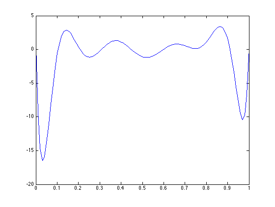
x = 0:0.1:1;
y = randn(1,11);
u = linspace(0,1,100);

plot(u,MyLagrange(x,y,u))

A38-39

A38_39

A40

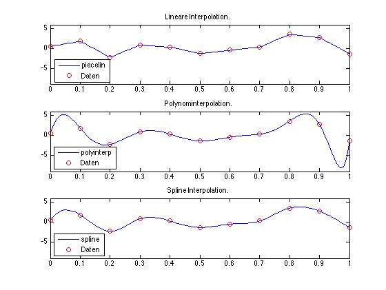
PlotInter

Published with MATLAB® R2014a

A38 + A39

clear all;

% Setze zu verwendende n.
N = 6:9;
% Runge-Funktion
f =@(x) 1./(1+x.^2);

% Definiere Vektor für den Plot.
X=linspace(-5,5,100);

% Farbauswahl max. 10
color = {'m','c','r','g','y','m-.','c-.','r-.','g-.','y-.'};

%cell für die Legende.
legendInfo=cell(length(N)+1,1);
% Plote exakte Lösung.
subplot(1,2,1);
plot(X,f(X),'k')
hold on;
legendInfo{1} = 'exact';

%Schleife über n.
for i = 1:length(N)
    x=linspace(-5,5,N(i));                  % n-Knoten
    y=f(x);                                 % n-Werte
    F = MyLagrange(x,y,X);                  % Interpoliere
    plot(X,F,color{i});                     % Plote
    legendInfo{i+1} = ['n = ' num2str(N(i))];  % Merke n für Legende.
end
legend(legendInfo) % erzeuge Legende
title('Äquidistante Knoten')
axis([-5 5 -1 1])
hold off

% Plote exakte Lösung in zweiten Plot.
subplot(1,2,2);
plot(X,f(X),'k')
hold on;
legendInfo{1} = 'exact';

ts=@(k,n) cos((2*k+1)./(2*n+2)*pi);

for i = 1:length(N)
    k=0:N(i)-1;                             % n-Knoten (-1) da
    x=ts(k,N(i)-1)*5.;                      % beginnend bei 0.
    y=f(x);                                 % n-Werte
    F = MyLagrange(x,y,X);                  % Interpoliere
    plot(X,F,color{i});                     % Plote
    legendInfo{i+1} = ['n = ' num2str(N(i))];  % Merke n für Legende.
end
legend(legendInfo) % erzeuge Legende
title('Tschebyschow Knoten')
axis([-5 5 -1 1])
hold off

Published with MATLAB® R2014a

function v = MyLagrange(x,y,u)
%Lagrange Interpolation.
%   v = MyLagrange(x,y,u) berechnet v(j) = P(u(j)) wobei P das
%   Interpolationspolynom vom Grad d = length(x)-1 mit
%   P(x(i)) = y(i) ist.


n = length(x);
v = zeros(size(u));

for k = 1:n  %Summe
   w = ones(size(u));
   for j = [1:k-1 k+1:n] %Produkt
      w = (u-x(j))./(x(k)-x(j)).*w;
   end
   v = v + w*y(k);
end

Published with MATLAB® R2014a

A40

clear all;

%Setze Daten x und f(x) = y
x = 0:0.1:1;
y = [ 0.5377    1.8339   -2.2588    0.8622    0.3188   -1.3077   ...
    -0.4336    0.3426    3.5784    2.7694   -1.3499];

%Definiere Vektor für den Plot.
u = linspace(0,1,100);

%Interpoliere
Fp = MyLagrange(x,y,u);
Fl = piecelin(x,y,u);
Fs = spline(x,y,u);

%Plote
subplot(3,1,1)
plot(u,Fl,'b',x,y,'ro')
title('Lineare Interpolation.')
legend('piecelin','Daten','Location','southwest')
axis([0 1 -9 6])

subplot(3,1,2)
plot(u,Fp,'b',x,y,'ro')
title('Polynominterpolation.')
legend('polyinterp','Daten','Location','southwest')
axis([0 1 -9 6])

subplot(3,1,3)
plot(u,Fs,'b',x,y,'ro')
title('Spline Interpolation.')
legend('spline','Daten','Location','southwest')
axis([0 1 -9 6])

Published with MATLAB® R2014a