Contents

Vorlesung 7: Graphik

clear all;
format short;

Die graphische Darstellung gehoert zu den Staerken von Matlab.

Graphische Darstellung von Funktionen / Daten

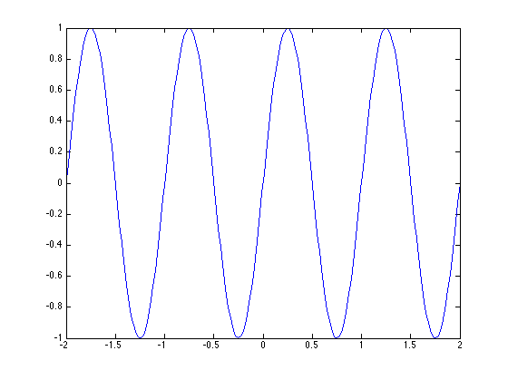
Bsp: zeichne die Funktion f(x) = cos(2 pi x) ueber dem Intervall [-2,2]

x = linspace(-2,2,200);
y = sin(2*pi*x);
plot(x,y);

help plot

 PLOT   Linear plot. 
    PLOT(X,Y) plots vector Y versus vector X. If X or Y is a matrix,
    then the vector is plotted versus the rows or columns of the matrix,
    whichever line up.  If X is a scalar and Y is a vector, disconnected
    line objects are created and plotted as discrete points vertically at
    X.
 
    PLOT(Y) plots the columns of Y versus their index.
    If Y is complex, PLOT(Y) is equivalent to PLOT(real(Y),imag(Y)).
    In all other uses of PLOT, the imaginary part is ignored.
 
    Various line types, plot symbols and colors may be obtained with
    PLOT(X,Y,S) where S is a character string made from one element
    from any or all the following 3 columns:
 
           b     blue          .     point              -     solid
           g     green         o     circle             :     dotted
           r     red           x     x-mark             -.    dashdot 
           c     cyan          +     plus               --    dashed   
           m     magenta       *     star             (none)  no line
           y     yellow        s     square
           k     black         d     diamond
           w     white         v     triangle (down)
                               ^     triangle (up)
                               <     triangle (left)
                               >     triangle (right)
                               p     pentagram
                               h     hexagram
                          
    For example, PLOT(X,Y,'c+:') plots a cyan dotted line with a plus 
    at each data point; PLOT(X,Y,'bd') plots blue diamond at each data 
    point but does not draw any line.
 
    PLOT(X1,Y1,S1,X2,Y2,S2,X3,Y3,S3,...) combines the plots defined by
    the (X,Y,S) triples, where the X's and Y's are vectors or matrices 
    and the S's are strings.  
 
    For example, PLOT(X,Y,'y-',X,Y,'go') plots the data twice, with a
    solid yellow line interpolating green circles at the data points.
 
    The PLOT command, if no color is specified, makes automatic use of
    the colors specified by the axes ColorOrder property.  By default,
    PLOT cycles through the colors in the ColorOrder property.  For
    monochrome systems, PLOT cycles over the axes LineStyleOrder property.
 
    Note that RGB colors in the ColorOrder property may differ from
    similarly-named colors in the (X,Y,S) triples.  For example, the 
    second axes ColorOrder property is medium green with RGB [0 .5 0],
    while PLOT(X,Y,'g') plots a green line with RGB [0 1 0].
 
    If you do not specify a marker type, PLOT uses no marker. 
    If you do not specify a line style, PLOT uses a solid line.
 
    PLOT(AX,...) plots into the axes with handle AX.
 
    PLOT returns a column vector of handles to lineseries objects, one
    handle per plotted line. 
 
    The X,Y pairs, or X,Y,S triples, can be followed by 
    parameter/value pairs to specify additional properties 
    of the lines. For example, PLOT(X,Y,'LineWidth',2,'Color',[.6 0 0]) 
    will create a plot with a dark red line width of 2 points.
 
    Example
       x = -pi:pi/10:pi;
       y = tan(sin(x)) - sin(tan(x));
       plot(x,y,'--rs','LineWidth',2,...
                       'MarkerEdgeColor','k',...
                       'MarkerFaceColor','g',...
                       'MarkerSize',10)
 
    See also PLOTTOOLS, SEMILOGX, SEMILOGY, LOGLOG, PLOTYY, PLOT3, GRID,
    TITLE, XLABEL, YLABEL, AXIS, AXES, HOLD, LEGEND, SUBPLOT, SCATTER.

    Overloaded methods:
       timeseries/plot

    Reference page in Help browser
       doc plot

Achsen

Matlab waehlt die Achsen automatisch basierend auf den Daten.

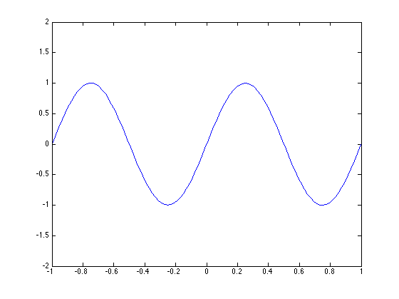
Wir koennen die Achsen auch explizit angeben, z.B. durch Eingabe von

plot(x,y);
axis([-1 1 -2 2])

Wir koennen auch die x- und y-Achse separat angeben:

plot(x,y);
xlim = [-2 2];
ylim = [-1 1];

Bildformat (aspect ratio)

plot(x,y)
daspect([1 1 1])

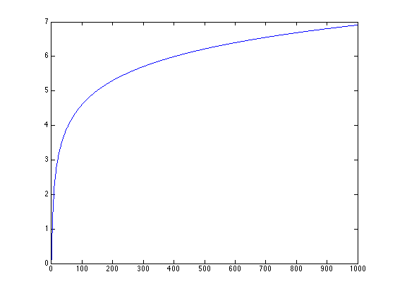
Logarithmische Skalierung

close all;
x = 0:1000;
y = log(x);
plot(x,y);

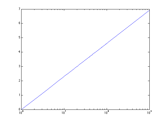
Logarithmische Skala der x-Achse

close all;
semilogx(x,y)

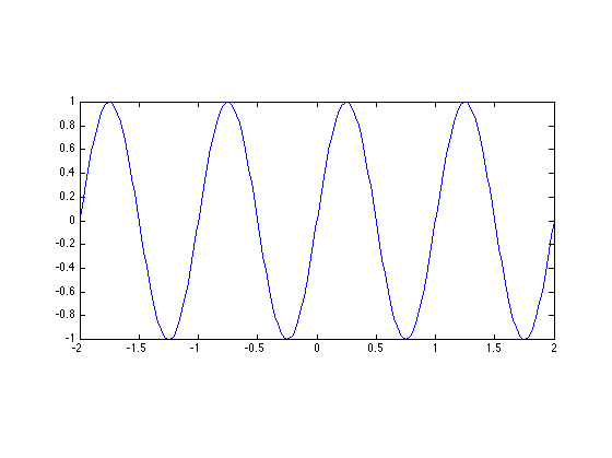
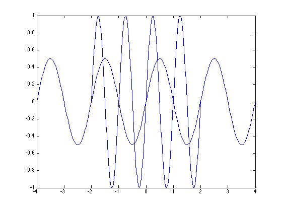
Gleichzeitige Darstellung mehrerer Funktionen

x = linspace(-2,2,200);
y = sin(2*pi*x);
close all;
plot(x,y);
hold on;
plot(2*x,y/2)

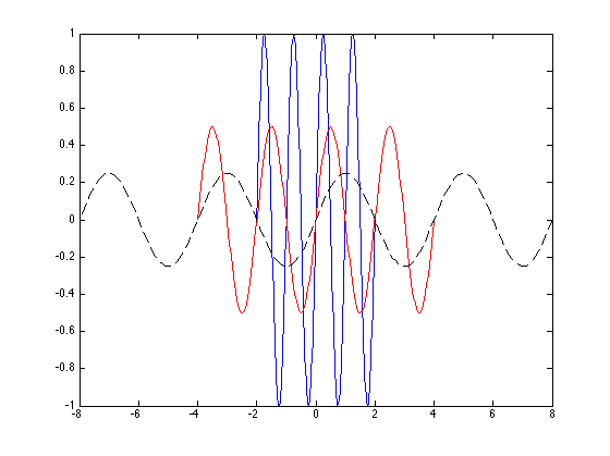
Auswahl von Farben und Linienarten

close all;
plot(x,y,'b')
hold on
plot(2*x,y/2,'r')
plot(4*x,y/4,'k--')

Zusaetzliche Markierungen

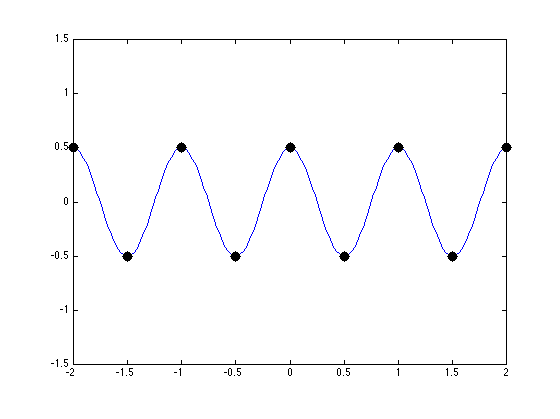
Beispiel: Zeichne die Funktion g(x) = cos(2 pi x) ueber dem Intervall [-2,2] und markiere Maxima und Minima der Funktion.

close all;
clear all;
x = linspace(-2,2,200);
g = @(x) cos(2*pi*x)/2;

plot(x,g(x))
xminmax = [-2:0.5:2];
hold on
plot(xminmax,g(xminmax),'k.','markersize',30)
axis([-2 2 -1.5 1.5])
daspect([1,1,1])

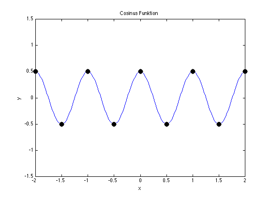
Bildueberschrift und Achsenbezeichnung

xlabel('x')
ylabel('y')
title('Cosinus Funktion')

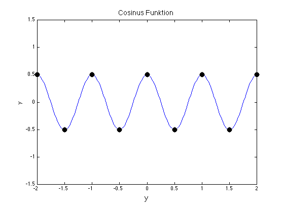
Schriftgroesse veraendern:

xlabel('x','FontSize',14);
xlabel('y','FontSize',14);
title('Cosinus Funktion','FontSize',14)

Abspeichern / Exportieren

Man kann das Figure als *.fig File abspeichern und zu einem spaeteren Zeitpunkt weiter verarbeiten.

saveas(gcf,'myfig.fig')

Dieses Bild koennen wir zu einem spaeteren Zeitpunkt oeffnen, dazu verwendet man

open myfig.fig

Ausserdem kann man das Fenster abspeichern um das Bild in ein anderes Dokumenten (Latex, Word) einzubinden.

help print

Beispiel:

print -depsc2 Cosinus.eps

Darstellung von 3D Daten

Verwendung von meshgrid

close all;
x = pi*(0:0.02:1);
y = 2*x;
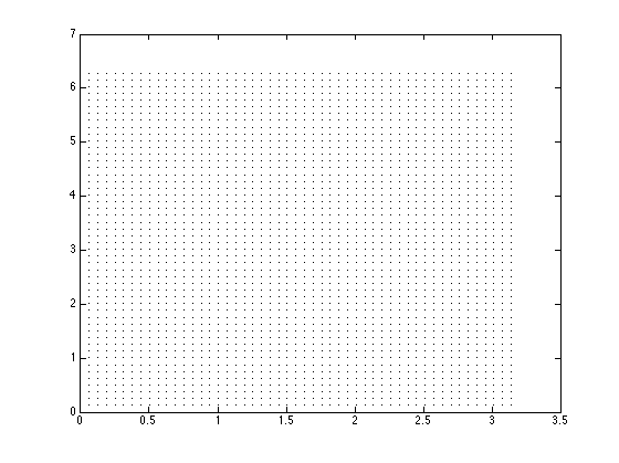
[X,Y] = meshgrid(x,y);

Die Felder X,Y definieren ein 2D Gitter

plot(X,Y,'k.')

Wir koennen ueber diesem Gitter Daten definieren.

Z = sin(X.^2+Y);
mesh(X,Y,Z)

Ersetze mesh durch surf , pcolor , contour

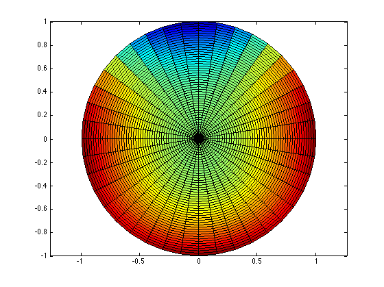
Obwohl die Daten ueber einem Rechtecksgitter definiert werden, koennen wir nicht nur Daten ueber rechteckigen Gebieten darstellen.

close all;
[R,T] = meshgrid(0:0.02:1,pi*(-1:0.05:1));
X = R.*cos(T);
Y = R.*sin(T);
pcolor(X,Y,X.^2-Y.^3);
axis equal

Clear und Close Graphic

clc % clear figure

close all

close(1)

EZ Plots

Easy to use function plotter

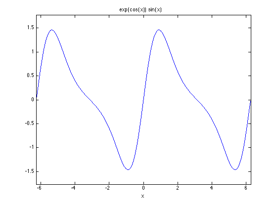
In der einfachsten Form benoetigt ezplot nur ein function handle Es wird dann die Funktion ueber dem Intervall [-2pi,2pi] gezeichnet.

clear all;
close all;
f = @(x) exp(cos(x)).*sin(x)

ezplot(f)

f = 

    @(x)exp(cos(x)).*sin(x)

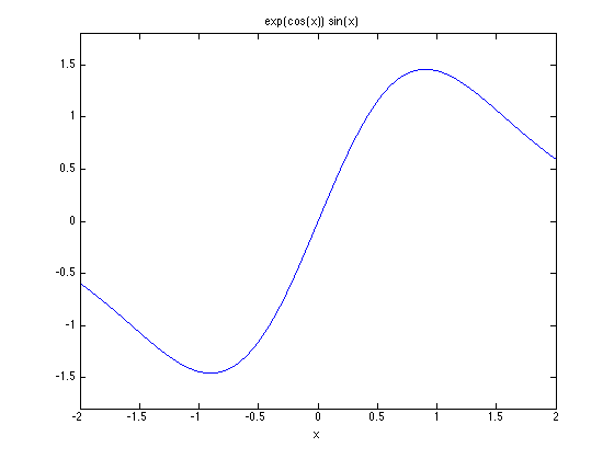
Angabe eines Intervalls

ezplot(f,[-2,2])
ezplot(f,[-2,2])

Weitere Beispiele zur Verwendung von ezplot

2D Plots expliziter und impliziter Funktionen; parametrischer Funktionen

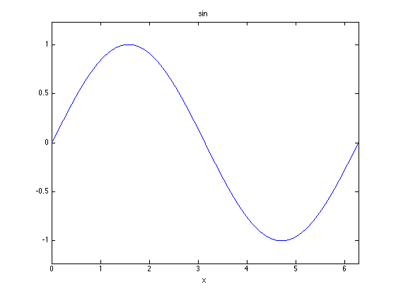
explizite Funktion y = f(x)

close all;
ezplot(@sin,[0,2*pi])

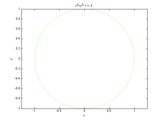
implizite Funktion F(x,y) = 0

close all;
ezplot(@(x,y) x.^2 + y.^2-1,[-1,1,-1,1])
axis equal

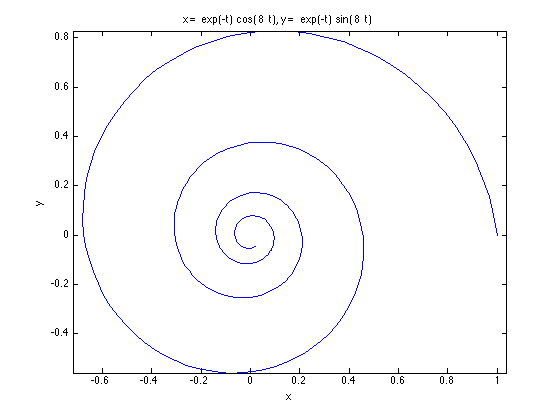
parametrische Funktion x = f(t), y = g(t)

close all;
x = @(t) exp(-t).*cos(8*t);
y = @(t) exp(-t).*sin(8*t);
ezplot(x,y,[0 3])

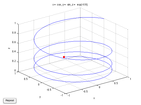
paramerische Raumkurven; 'animate' ein Ablaufen der Raumkurve

close all;
ezplot3(@cos,@sin,@(t) exp(-t/8),[0,20],'animate')

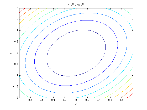
Contourplots

Plotte eine Familie von Kurven f(x,y) = c in der x-y-Ebene fuer verschiedene Werte von c.

close all;
ezcontour(@(x,y) 4*x.^2-x.*y+y.^2, [-1 1 -2 2])

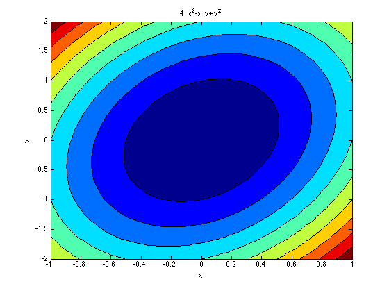
close all;
ezcontourf(@(x,y) 4.*x.^2-x.*y+y.^2,[-1 1 -2 2])

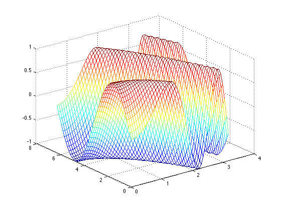
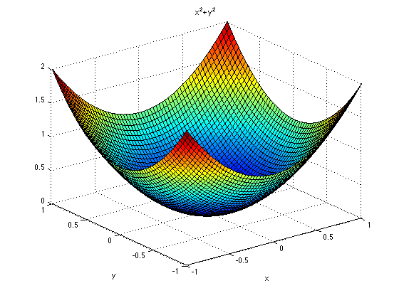
Surfaceplot

explizite Oberflaeche z = F(x,y)

close all;
ezsurf(@(x,y) x.^2 + y.^2,[-1 1 -1 1])

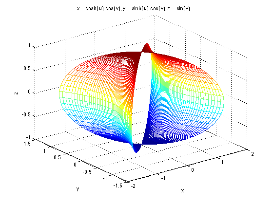
parameter Plot

close all;
x = @(u,v) cosh(u).*cos(v);
y = @(u,v) sinh(u).*cos(v);
z = @(u,v) sin(v);
ezmesh(x,y,z,[-1 1 0 2*pi])

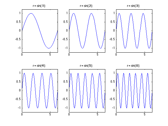
Subplots

close all;
for n=1:6
    subplot(2,3,n), ezplot(@(t) sin(n*t),[0 2*pi])
    xlabel('');
    title(['r = sin(',int2str(n),'t)'])
end

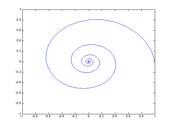
Animation

close all;
t=linspace(0,8*pi,800)';
for s=0:0.01:1
    x = exp(-s*t).*cos(6*s*t+t);
    y = exp(-s*t).*sin(6*s*t+t);
    plot(x,y);
    axis([-1 1 -1 1]);
    pause(0.01)
end

Published with MATLAB® R2014a