Contents

6. Vorlesung: Funktionen

Bisher haben wir ein Matlab-Script geschrieben, um eine gegebene Aufgabenstellung mit Matlab zu loesen. Der wesentliche Unterschie zwischen einem Script und einer function ist der lokale Workspace .

Alle Variablen die waehrend der Ausfuehrung einer function erzeugt werden, sind nur innerhalb dieses Funktionsaufrufs verfuegbar. Andererseits sind die Variablen des Basis Workspace (d.h. die, die auf der Ebene der Kommandozeile bekannt sind), nicht innerhalb einer function bekannt.

Funktionen werden als m-File abgespeichert. Der Name des m-Files entspricht dem Funktionsnamen.

% quadform.m ist separate Funktion
%
[r1,r2] = quadform(1,1,1);
fprintf('erste Nullstelle:');
display(r1);

fprintf('zweite Nullstelle:');
display(r2);

erste Nullstelle:
r1 =

  -0.5000 + 0.8660i

zweite Nullstelle:
r2 =

  -0.5000 - 0.8660i

function handles

Oft moechte man eine Funktion schreiben oder benutzen, die eine andere Funktion als Eingangsargument enthaelt.

Matlab-Bezeichnung: function functions

Beispiele:

help funfun

  Function functions and ODE solvers.
 
  Numerical integration (quadrature).
    integral   - Numerically evaluate integral.
    integral2  - Numerically evaluate double integral.
    integral3  - Numerically evaluate triple integral.
    quad       - Numerically evaluate integral, low order method.
    quadgk     - Numerically evaluate integral, adaptive Gauss-Kronrod quadrature.
    quadl      - Numerically evaluate integral, higher order method.
    quadv      - Vectorized QUAD.
    quad2d     - Numerically evaluate double integral over a planar region.
    dblquad    - Numerically evaluate double integral over a rectangle.
    triplequad - Numerically evaluate triple integral.
 
  Plotting.
    ezplot     - Easy to use function plotter.
    ezplot3    - Easy to use 3-D parametric curve plotter.
    ezpolar    - Easy to use polar coordinate plotter.
    ezcontour  - Easy to use contour plotter.
    ezcontourf - Easy to use filled contour plotter.
    ezmesh     - Easy to use 3-D mesh plotter.
    ezmeshc    - Easy to use combination mesh/contour plotter.
    ezsurf     - Easy to use 3-D colored surface plotter.
    ezsurfc    - Easy to use combination surf/contour plotter.
    fplot      - Plot function.
 
  Inline function object.
    inline     - Construct INLINE function object.
    argnames   - Argument names.
    formula    - Function formula.
    char       - Convert INLINE object to character array.
 
  Differential equation solvers.
  Initial value problem solvers for ODEs. (If unsure about stiffness, try ODE45
  first, then ODE15S.)
    ode45     - Solve non-stiff differential equations, medium order method.
    ode23     - Solve non-stiff differential equations, low order method.
    ode113    - Solve non-stiff differential equations, variable order method.
    ode23t    - Solve moderately stiff ODEs and DAEs Index 1, trapezoidal rule.
    ode15s    - Solve stiff ODEs and DAEs Index 1, variable order method.
    ode23s    - Solve stiff differential equations, low order method.
    ode23tb   - Solve stiff differential equations, low order method.
 
  Initial value problem solver for fully implicit ODEs/DAEs F(t,y,y')=0.
    decic     - Compute consistent initial conditions.
    ode15i    - Solve implicit ODEs or DAEs Index 1.
 
  Initial value problem solver for delay differential equations (DDEs). 
    dde23     - Solve delay differential equations (DDEs) with constant delays.
    ddesd     - Solve delay differential equations (DDEs) with variable delays.
    ddensd    - Solve delay differential equations (DDEs) of neutral type.
 
  Boundary value problem solver for ODEs.
    bvp4c     - Solve boundary value problems by collocation, 3-stage Lobatto formula.
    bvp5c     - Solve boundary value problems by collocation, 4-stage Lobatto formula.
 
  1D Partial differential equation solver.
    pdepe     - Solve initial-boundary value problems for parabolic-elliptic PDEs.
  
  Option handling.
    odeset    - Create/alter ODE OPTIONS structure.
    odeget    - Get ODE OPTIONS parameters.
    ddeset    - Create/alter DDE OPTIONS structure.
    ddeget    - Get DDE OPTIONS parameters.
    bvpset    - Create/alter BVP OPTIONS structure.
    bvpget    - Get BVP OPTIONS parameters.
 
  Input and Output functions.
    deval     - Evaluates the solution of a differential equation problem.
    odextend  - Extends the solutions of a differential equation problem.
    odeplot   - Time series ODE output function.
    odephas2  - 2-D phase plane ODE output function.
    odephas3  - 3-D phase plane ODE output function.
    odeprint  - Command window printing ODE output function.
    bvpinit   - Forms the initial guess for BVP4C and BVP5C.
    bvpxtend  - Forms a guess structure for extending BVP solution. 
    pdeval    - Evaluates by interpolation the solution computed by PDEPE.

Integration

help integral

 INTEGRAL  Numerically evaluate integral.
    Q = INTEGRAL(FUN,A,B) approximates the integral of function FUN from A
    to B using global adaptive quadrature and default error tolerances.
 
    FUN must be a function handle. A and B can be -Inf or Inf. If both are
    finite, they can be complex. If at least one is complex, INTEGRAL
    approximates the path integral from A to B over a straight line path.
 
    For scalar-valued problems the function Y = FUN(X) must accept a vector
    argument X and return a vector result Y, the integrand function
    evaluated at each element of X. For array-valued problems (see the
    'ArrayValued' option below) FUN must accept a scalar and return an
    array of values.
 
    Q = INTEGRAL(FUN,A,B,PARAM1,VAL1,PARAM2,VAL2,...) performs the
    integration with specified values of optional parameters. The available
    parameters are
 
    'AbsTol', absolute error tolerance
    'RelTol', relative error tolerance
 
        INTEGRAL attempts to satisfy |Q - I| <= max(AbsTol,RelTol*|Q|),
        where I denotes the exact value of the integral. Usually RelTol
        determines the accuracy of the integration. However, if |Q| is
        sufficiently small, AbsTol determines the accuracy of the
        integration, instead. The default value of AbsTol is 1.e-10, and
        the default value of RelTol is 1.e-6. Single precision integrations
        may require larger tolerances.
 
    'ArrayValued', FUN is an array-valued function when the input is scalar
 
        When 'ArrayValued' is true, FUN is only called with scalar X, and
        if FUN returns an array, INTEGRAL computes a corresponding array of
        outputs Q. The default value is false.
 
    'Waypoints', vector of integration waypoints
 
        If FUN(X) has discontinuities in the interval of integration, the
        locations should be supplied as a 'Waypoints' vector. Waypoints
        should not be used for singularities in FUN(X). Instead, split the
        interval and add the results from separate integrations with
        singularities at the endpoints. If A, B, or any entry of the
        waypoints vector is complex, the integration is performed over a
        sequence of straight line paths in the complex plane, from A to the
        first waypoint, from the first waypoint to the second, and so
        forth, and finally from the last waypoint to B.
 
    Examples:
        % Integrate f(x) = exp(-x^2)*log(x)^2 from 0 to infinity:
        f = @(x) exp(-x.^2).*log(x).^2
        Q = integral(f,0,Inf)
 
        % To use a parameter in the integrand:
        f = @(x,c) 1./(x.^3-2*x-c)
        Q = integral(@(x)f(x,5),0,2)
 
        % Specify tolerances:
        Q = integral(@(x)log(x),0,1,'AbsTol',1e-6,'RelTol',1e-3)
 
        % Integrate f(z) = 1/(2z-1) in the complex plane over the
        % triangular path from 0 to 1+1i to 1-1i to 0:
        Q = integral(@(z)1./(2*z-1),0,0,'Waypoints',[1+1i,1-1i])
 
        % Integrate the vector-valued function sin((1:5)*x) from 0 to 1:
        Q = integral(@(x)sin((1:5)*x),0,1,'ArrayValued',true)
 
    Class support for inputs A, B, and the output of FUN:
       float: double, single
 
    See also INTEGRAL2, INTEGRAL3, FUNCTION_HANDLE

    Reference page in Help browser
       doc integral

Beispiel:

integral(sin,0,pi) % erzeugt eine Fehlermeldung

integral(@sin,0,pi)

ans =

    2.0000

Anonymous function

Eine anonymous function definiert gleichzeitig eine Funktion und erzeugt ein handle.

Beispiel:

sincos = @(x) sin(x) + cos(x);
integral(sincos,0,pi)

ans =

     2

Alternativ:

integral(@(x) sin(x)+cos(x),0,pi)

ans =

     2

Nullstellenbestimmung

help fzero

 FZERO  Single-variable nonlinear zero finding. 
    X = FZERO(FUN,X0) tries to find a zero of the function FUN near X0, 
    if X0 is a scalar.  It first finds an interval containing X0 where the 
    function values of the interval endpoints differ in sign, then searches 
    that interval for a zero.  FUN is a function handle.  FUN accepts real 
    scalar input X and returns a real scalar function value F, evaluated 
    at X. The value X returned by FZERO is near a point where FUN changes 
    sign (if FUN is continuous), or NaN if the search fails.  
 
    X = FZERO(FUN,X0), where X0 is a vector of length 2, assumes X0 is a 
    finite interval where the sign of FUN(X0(1)) differs from the sign of 
    FUN(X0(2)). An error occurs if this is not true.  Calling FZERO with a
    finite interval guarantees FZERO will return a value near a point where
    FUN changes sign.
 
    X = FZERO(FUN,X0), where X0 is a scalar value, uses X0 as a starting 
    guess. FZERO looks for an interval containing a sign change for FUN and 
    containing X0.  If no such interval is found, NaN is returned.  
    In this case, the search terminates when the search interval 
    is expanded until an Inf, NaN, or complex value is found. Note: if
    the option FunValCheck is 'on', then an error will occur if an NaN or 
    complex value is found.
 
    X = FZERO(FUN,X0,OPTIONS) solves the equation with the default optimization
    parameters replaced by values in the structure OPTIONS, an argument
    created with the OPTIMSET function.  See OPTIMSET for details.  Used
    options are Display, TolX, FunValCheck, OutputFcn, and PlotFcns. 
 
    X = FZERO(PROBLEM) finds the zero of a function defined in PROBLEM. 
    PROBLEM is a structure with the function FUN in PROBLEM.objective, 
    the start point in PROBLEM.x0, the options structure in PROBLEM.options,
    and solver name 'fzero' in PROBLEM.solver. The structure PROBLEM must have 
    all the fields.
 
    [X,FVAL]= FZERO(FUN,...) returns the value of the function described 
    in FUN, at X.
 
    [X,FVAL,EXITFLAG] = FZERO(...) returns an EXITFLAG that describes the 
    exit condition of FZERO. Possible values of EXITFLAG and the corresponding 
    exit conditions are
 
      1  FZERO found a zero X.
     -1  Algorithm terminated by output function.
     -3  NaN or Inf function value encountered during search for an interval
          containing a sign change.
     -4  Complex function value encountered during search for an interval 
          containing a sign change.
     -5  FZERO may have converged to a singular point.
     -6  FZERO can not detect a change in sign of the function.
 
    [X,FVAL,EXITFLAG,OUTPUT] = FZERO(...) returns a structure OUTPUT
    with the number of function evaluations in OUTPUT.funcCount, the
    algorithm name in OUTPUT.algorithm, the number of iterations to
    find an interval (if needed) in OUTPUT.intervaliterations, the
    number of zero-finding iterations in OUTPUT.iterations, and the
    exit message in OUTPUT.message.
 
    Examples
      FUN can be specified using @:
         X = fzero(@sin,3)
      returns pi.
         X = fzero(@sin,3,optimset('Display','iter')) 
      returns pi, uses the default tolerance and displays iteration information.
 
      FUN can be an anonymous function:
         X = fzero(@(x) sin(3*x),2)
 
      FUN can be a parameterized function.  Use an anonymous function to
      capture the problem-dependent parameters:
         myfun = @(x,c) cos(c*x);  % The parameterized function.
         c = 2;                    % The parameter.
         X = fzero(@(x) myfun(x,c),0.1)
    
    Limitations
         X = fzero(@(x) abs(x)+1, 1) 
      returns NaN since this function does not change sign anywhere on the 
      real axis (and does not have a zero as well).
         X = fzero(@tan,2)
      returns X near 1.5708 because the discontinuity of this function near the 
      point X gives the appearance (numerically) that the function changes sign at X.
 
    See also ROOTS, FMINBND, FUNCTION_HANDLE.

    Reference page in Help browser
       doc fzero

Wir wollen eine Nullstelle der Funktion sin(x)+cos(x) bestimmen. Zunaechst zeichnen wir die Funktion.

x = linspace(0,2*pi,1000);
plot(x,sincos(x))

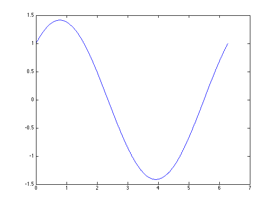
Wir nutzen 2.5 als Startwert fuer die Nullstellensuche.

fzero(sincos,2.5)

ans =

    2.3562

Beispiel fuer eine anonyme Funktion mit mehreren Argumenten:

w = @(x,t) sin(x+t);

Berechne Nullstelle fuer Verschiedene Werte von t.

for t=0:0.25:2
    x0 = fzero(@(x) sin(x+t),0);
    fprintf('Nullstelle von sin(x+%1.2f): %f\n',t,x0);
end

Nullstelle von sin(x+0.00): 0.000000
Nullstelle von sin(x+0.25): -0.250000
Nullstelle von sin(x+0.50): -0.500000
Nullstelle von sin(x+0.75): -0.750000
Nullstelle von sin(x+1.00): -1.000000
Nullstelle von sin(x+1.25): -1.250000
Nullstelle von sin(x+1.50): -1.500000
Nullstelle von sin(x+1.75): -1.750000
Nullstelle von sin(x+2.00): 1.141593

Unterfunktionen und eingebettete Funktionen

Betrachte quadform2.m als Beispiel fuer eine Funktion mit Unterfunktion.

Betrachte quadform2.m

[r1,r2]=quadform2(1,1,1)

r1 =

  -0.5000 + 0.8660i


r2 =

  -0.5000 - 0.8660i

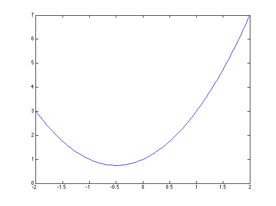
Erzeugung eines function handle fuer eine eingebettete Funktion.

Betrachte makeParabola.m

p = makeParabel(1,1,1);
x = linspace(-2,2,100);
y = p(x);
plot(x,y)

Rekursive Funktionen

Wie in verschiedenen anderen Programmiersprachen koennen Funktionsaufrufe in Matlab auch rekursiv sein. Dies bedeutet, dass eine Funktion sich selbst im Inneren aufrufen darf. Dies birgt natuerlich die Gefahr von unendlichen Schleifen. Um dem vorzubegen sind rekursive Funktionen streng an drei elementare Regeln gebunden.

Beispiel: Betrachte fakrec.m.

fakrekur(3)

ans =

     6

Published with MATLAB® R2014a

% Refursive Funktion zur Berechnung der Fakultaet.
function fw = fakrekur(n)
  if n <=1
      fw = 1;
  else
      fw = n*fakrekur(n-1);
  end
end

Published with MATLAB® R2014a

function p = makeParabel(a,b,c)
p = @parabel;

    function y = parabel(x)
        y = a*x.^2 + b*x + c;
    end

end

Published with MATLAB® R2014a

function [x1,x2] = quadform(a,b,c)

d = sqrt(b^2 - 4*a*c);
x1 = (-b+d) / (2*a);
x2 = (-b-d) / (2*a);
end

Published with MATLAB® R2014a

function [x1,x2] = quadform2(a,b,c)
d = discrim(a,b,c);
x1 = (-b+d) / (2*a);
x2 = (-b-d) / (2*a);
end
function D = discrim(A,B,C)
D = sqrt(B^2 - 4*A*C);
end

Published with MATLAB® R2014a