Contents

VL11: Ausgleichsrechnung

clear all;
close all;

t = (0:0.01:3)';
y = 4 + cos(t) - 0.5*sin(t)+0.2*rand(size(t));
plot(t,y,'r.')

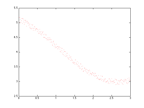
Ziel: Bestimme eine Kurve, die diese Daten gut approximiert.

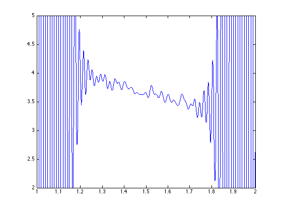
1. Versuch: Polynominterpolation

close all;
tt = 0:0.001:3;
yy = polyinterp(t,y,tt);
plot(t,y,'r.')
hold on
plot(tt,yy)
axis([1 2 2 5])
hold off

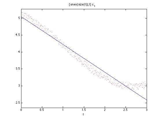
2. Versuch: Berechne Ausgleichsgrade

X1 = [ones(size(t)) t];
c1 = X1\y;
f1 = @(t) [ones(size(t)) t]*c1;
close all
plot(t,y,'r.');
hold on
ezplot(f1,[0,3])

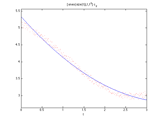
3. Versuch: Berechne Polynom

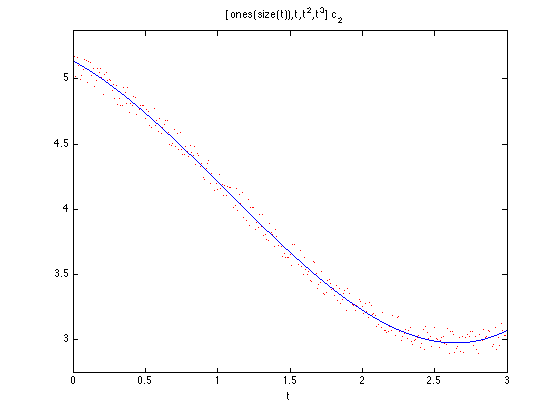
X2 = [ones(size(t)) t t.^2];
c2 = X2\y;
f2 = @(t) [ones(size(t)) t t.^2]*c2;
close all
plot(t,y,'r.');
hold on
ezplot(f2,[0,3])

X2 = [ones(size(t)) t t.^2 t.^3];
c2 = X2\y;
f2 = @(t) [ones(size(t)) t t.^2 t.^3]*c2;
close all
plot(t,y,'r.');
hold on
ezplot(f2,[0,3])

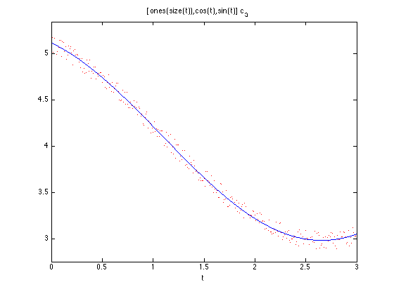
4. Versuch: Benutze die Basis 1, sin(t), cos(t):

X3 = [ones(size(t)) cos(t) sin(t)];
c3 = X3\y;

f = @(t) [ones(size(t)) cos(t) sin(t)]*c3;
close all
plot(t,y,'r.');
hold on;
ezplot(f,[0 3])

Verwende QR-Zerlegung

X4 = [ones(size(t)) cos(t) sin(t)];
[Q,R]=qr(X4,0);
c4 = R\(Q'*y);
f = @(t) [ones(size(t)) cos(t) sin(t)]*c4;
close all;
plot(t,y,'r.');
hold on;
ezplot(f,[0,3])

Veranschaulichung der Funktionsweise von qr(X,y)

t = (0:0.25:1)';
y = 4 + cos(t) - 0.5*sin(t)+0.2*rand(size(t));
X = [ones(size(t)) cos(t) sin(t)];
qrsteps(X,y)

A =

    1.0000    1.0000         0
    1.0000    0.9689    0.2474
    1.0000    0.8776    0.4794
    1.0000    0.7317    0.6816
    1.0000    0.5403    0.8415


b =

    5.1364
    4.8537
    4.6522
    4.4952
    4.1389


A =

   -2.2361   -1.8418   -1.0062
         0    0.0907   -0.0635
         0   -0.0006    0.1685
         0   -0.1465    0.3707
         0   -0.3379    0.5305


b =

  -10.4095
    0.0497
   -0.1518
   -0.3087
   -0.6650


A =

   -2.2361   -1.8418   -1.0062
         0   -0.3793    0.6313
         0         0    0.1676
         0         0    0.1542
         0         0    0.0311


b =

  -10.4095
   -0.7238
   -0.1508
   -0.0676
   -0.1089


A =

   -2.2361   -1.8418   -1.0062
         0   -0.3793    0.6313
         0         0   -0.2298
         0         0         0
         0         0         0


b =

  -10.4095
   -0.7238
    0.1701
    0.0568
   -0.0838


ans =

   -2.2361   -1.8418   -1.0062
         0   -0.3793    0.6313
         0         0   -0.2298
         0         0         0
         0         0         0

Published with MATLAB® R2014a

function v = polyinterp(x,y,u)
%POLYINTERP  Polynomial interpolation.
%   v = POLYINTERP(x,y,u) computes v(j) = P(u(j)) where P is the
%   polynomial of degree d = length(x)-1 with P(x(i)) = y(i).

% Use Lagrangian representation.
% Evaluate at all elements of u simultaneously.

n = length(x);
v = zeros(size(u));
for k = 1:n
   w = ones(size(u));
   for j = [1:k-1 k+1:n]
      w = (u-x(j))./(x(k)-x(j)).*w;
   end
   v = v + w*y(k);
end

Published with MATLAB® R2014a

function [A,b] = qrsteps(A,b)
%QRSTEPS  Orthogonal-triangular decomposition.
%   Demonstrates M-file version of built-in QR function.
%   R = QRSTEPS(A) is the upper trapezoidal matrix R that
%   results from the orthogonal transformation, R = Q'*A.
%   With no output argument, QRSTEPS(A) shows the steps in
%   the computation of R.  Press <enter> key after each step.
%   [R,bout]  = QRSTEPS(A,b) also applies the transformation to b.

[m,n] = size(A);
if nargin < 2, b = zeros(m,0); end

% Householder reduction to triangular form.

if nargout == 0
   clc
   A
   if ~isempty(b), b, end
   pause
end

for k = 1:min(m-1,n)
   % Introduce zeros below the diagonal in the k-th column.
   % Use Householder transformation, I - rho*u*u'.
   i = k:m;
   u = A(i,k);
   sigma = norm(u);

   % Skip transformation if column is already zero.
   if sigma ~= 0

      if u(1) ~= 0, sigma = sign(u(1))*sigma; end
      u(1) = u(1) + sigma;
      rho = 1/(conj(sigma)*u(1));

      % Update the k-th column.
      A(i,k) = 0;
      A(k,k) = -sigma;

      % Apply the transformation to remaining columns of A.
      j = k+1:n;
      v = rho*(u'*A(i,j));
      A(i,j) = A(i,j) - u*v;

      % Apply the transformation to b.
      if ~isempty(b)
         tau = rho*(u'*b(i));
         b(i) = b(i) - tau*u;
      end
   end
   if nargout == 0
      clc
      A
      if ~isempty(b), b, end
      pause
   end
end

Published with MATLAB® R2014a